






A Canadian data analyst time series portfolio should show more than a smooth chart. It should let another reader identify the measure, retrieve the source and understand what changed when the data were revised. That makes a small project useful even before it becomes a large dashboard.
Statistics Canada released its 2026 time-series guidelines on 13 November. The full guidance explains that new information can revise past adjusted estimates. It also gives context-specific history recommendations for identifying seasonal and calendar effects. Those points provide a practical foundation for a portfolio exercise.
Canadian data analyst time series portfolio: define one question
Choose a question that one well-defined series can answer. For example, a project might explain how a published measure changed between two reference periods and whether a later release changes that explanation. Keep the purpose narrow enough that you can document every transformation.
Record the population, geography, units, frequency and adjustment status before plotting. A monthly count and an annual rate do not become comparable because the dashboard places them side by side. Similarly, an adjusted series and its raw counterpart serve different questions. Preserve those labels in the data and the chart.
Translate years into observations carefully
Within its seasonal-adjustment framework, Statistics Canada recommends 10–15 years of history. It gives minima of five years for a seasonal pattern and seven for calendar effects. For a complete monthly series, those become 120–180, 60 and 84 observations respectively. Length alone does not establish suitability.
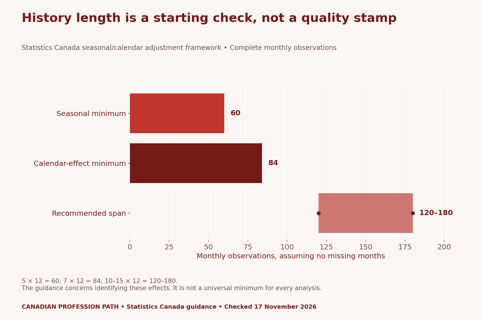
Use the conversion as a planning check, rather than a permission slip to run a model. Missing months, measurement changes and the question itself can still limit the analysis. If you use a shorter series for a descriptive exercise, state that narrower purpose. Do not claim that you have established a stable seasonal pattern.
Beginners can work with official adjusted data and explain its definitions. That is different from reproducing the agency’s production adjustment process. A notebook that downloads a published result should describe exactly that task. It should not imply that it replicated a full statistical production system.
Keep release time separate from reference time
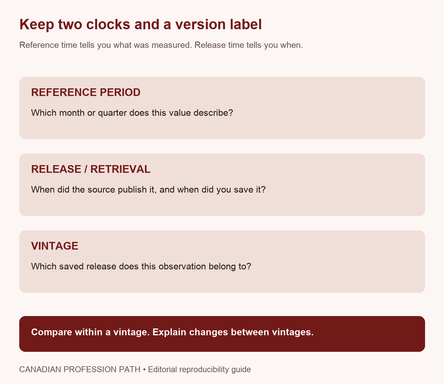
Create an immutable source folder for each retrieval. Give each file a clear vintage label and record its checksum. Then store transformations in a separate output folder. If a fresh download arrives, add another source file instead of replacing the first one. This preserves what a reader could have known at each release.
The blank register includes both release date and retrieval timestamp. They need not be identical. A file downloaded today may contain a release published earlier. If you cannot establish the source’s release date, leave that limitation visible. Do not quietly relabel the download time as the publication date.
Use a fictional revision example to test the logic
Consider two teaching values: an earlier period is 100 and a later period is 102. Their percentage change is (102 ÷ 100 − 1) × 100 = 2%. Now suppose a later vintage revises the earlier period to 103 while the later value remains 102. These are fictional values, not Canadian observations.
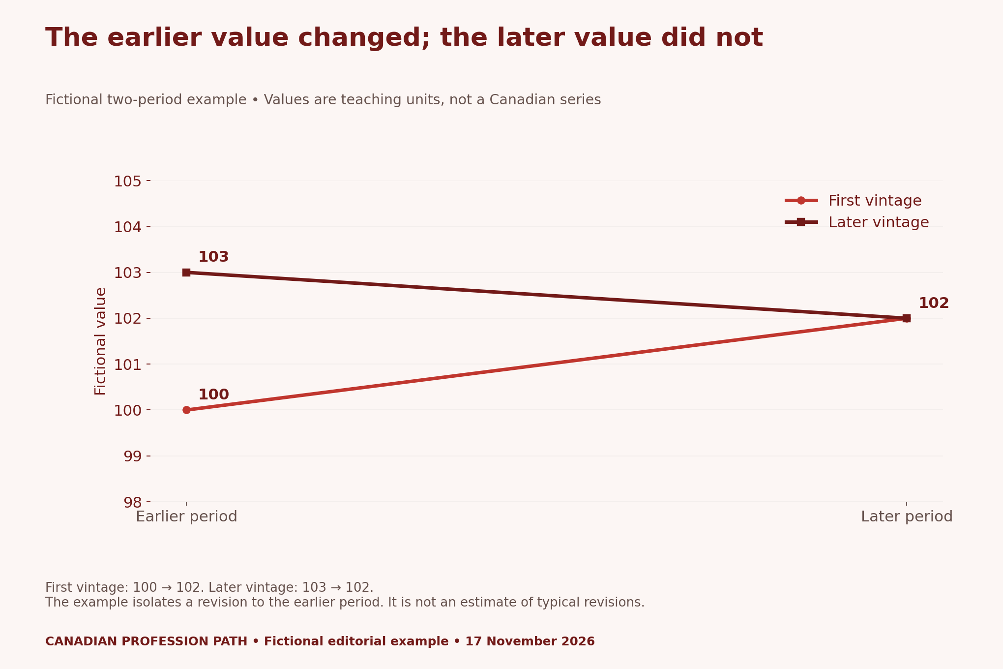
Using the later vintage consistently, the change is (102 ÷ 103 − 1) × 100, approximately −0.97%. The sign changes because the comparison’s starting value changes. The example demonstrates a denominator issue without pretending that a real Canadian indicator behaved this way.
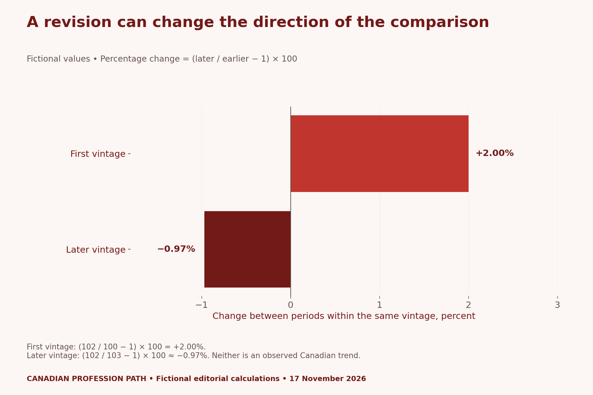
Do not combine the first vintage’s earlier value with the later vintage’s later value unless that mixed-vintage question is explicitly intended and labelled. Otherwise, the chart can hide which information set produced the result. Keep a reproducible calculation for each release, then explain the difference between releases separately.
Build a small dashboard with an audit trail
A useful design has a measure definition, a vintage selector and a short explanation of the calculation. Show the chosen source file beside the output. Let readers see which period and data version feed the chart. A visible revision note is more useful than an unexplained jump in a refreshed dashboard.
Add a decision log when the project changes. Record why you changed a unit, excluded a period or selected an adjusted series. Keep the original value intact and describe transformations in separate fields. Someone reviewing the project should be able to distinguish a source revision from an error you corrected in your own code.
Our Information Technology and Computer Science archive provides wider career context. For this exercise, the deliverable is evidence of careful analytical work. We have not tested whether this particular portfolio format improves hiring outcomes.
Explain the result to a nontechnical reader
Write a short note answering three questions: what did the chosen vintage show, what changed in the next vintage and what conclusion remains justified? Avoid calling every month-to-month movement a trend. Also avoid treating a revised estimate as evidence that the earlier release was dishonest or useless.
A portfolio can acknowledge uncertainty while remaining clear. Use a concrete sentence about the actual comparison and place its limitation nearby. If a break in definition prevents a valid comparison, say so. An attractive graphic cannot repair a change in the statistical concept being measured.
Method, limitations and downloadable tools
We checked the November 13 guidance on 17 November 2026. The history conversions assume twelve observations per year. The revision figures use an explicitly fictional two-period dataset with full arithmetic in the CSV. No Canadian time-series dataset, completed dashboard, production adjustment replication or hiring experiment is claimed.
- Guideline spans and monthly-observation conversions (CSV)
- Fictional vintage values and percentage calculations (CSV)
- Blank source, metadata and vintage register (CSV)
- Revision-aware notebook and communication checklist (CSV)
Suggested citation: Canadian Profession Path, “Canadian Data Analyst Portfolio: Show That Your Trend Survives Revisions”, 17 November 2026. Source: Statistics Canada time-series guidelines; conversions, fictional examples and planning tools by the publication.


